CNR-calibrated correction restores accuracy
Joseph J. Thiebes, Marc Meléndez, Enrique Arévalo Rodríguez, Ferry Prins
Condensed Matter Physics Center (IFIMAC), Universidad Autónoma de Madrid
Departamento de Física de la Materia Condensada, Facultad de Ciencias, Universidad Autónoma de Madrid
Presented at the Gordon Research Seminar and Gordon Research Conference on Colloidal Nanocrystals
Les Diablerets, Switzerland, July 4–10, 2026.
The problem: a width can’t go negative
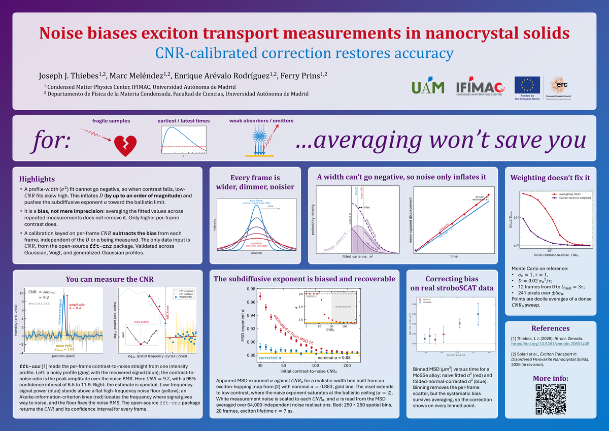
Transport microscopy extracts diffusion parameters from the frame-by-frame broadening of an excited-state population: fit a profile width σ² at each time delay, form the mean-squared displacement (MSD), and measure the diffusion coefficient D or the transport exponent α from its slope. The width fit is bounded at zero, because a width cannot be negative. When contrast falls, the estimator’s distribution piles up against that bound and skews high, so low-CNR fits can only err upward. The result is an inflated D, by up to an order of magnitude, and an apparent α biased toward the ballistic limit.
This is a bias, not a loss of precision: averaging fitted values across repeated measurements does not remove it, and neither does inverse-variance weighting of the MSD. Because the signal decays over the measurement, every frame is wider, dimmer, and noisier than the last, so the bias grows with time delay and distorts the functional form of the MSD rather than shifting it uniformly. The regime is a common one: fragile samples, the earliest and latest time points of any decay, and weak absorbers or emitters.
Report the CNR, whatever regime you work in
The bias scales with contrast: negligible at high CNR, severe at low CNR. The CNR is therefore the quantity to report. Where measurements sit well above the noise, fft-cnr documents that margin for the methods section; where they sit closer to the noise floor than expected, the same measurement gives warning before the bias reaches the result. Either way, the reader gains a number to judge the measurement by, reported alongside the integration time and excitation power already reported, at the cost of a single function call.
fft-cnr is an open-source Python package that measures the CNR of a 1-D profile from a single acquisition, with no repeat frames and no separate background region. In the power spectrum, low-frequency signal power stands above a flat high-frequency noise floor; an Akaike-information-criterion knee locates the boundary between them, and the package returns the CNR with a 95% confidence interval. It also detects when noise is signal-dependent (the shot-noise regime, where the naive CNR overstates the true peak SNR) and reports a corrected value, flags frames where a low-frequency baseline or an opposite-sign feature makes the amplitude ambiguous, and returns the fitted profile parameters — center, width, and shape — when those are wanted alongside the contrast. Installation is pip install fft-cnr; the CNR of a profile is fft_cnr(profile).cnr.
The bias correction uses that measurement. A calibration keyed on the per-frame CNR subtracts the width bias from each frame, independent of the D or α being measured; its only data input is the CNR. It is validated across Gaussian, Voigt (mixed Gaussian-Lorentzian), and generalized-Gaussian profile shapes.
Results
On a test bed built from an exciton-hopping map of a disordered perovskite nanocrystal solid (nominal α = 0.883; 250 × 250 spatial bins, 20 frames, 7 ns exciton lifetime, 64,000 independent noise realizations), the naive exponent climbs as CNR falls and saturates at the ballistic ceiling of α = 2: noise alone converts subdiffusion into apparent ballistic transport. The CNR-calibrated correction recovers the nominal exponent down into the low-contrast regime. Applied to real stroboSCAT data on a MoSSe alloy, the corrected width separates cleanly from the naive fit at every binned point: binning removes the frame-to-frame scatter, but the systematic bias survives averaging, so the correction is visible point by point.
Links
- Poster PDF: Download PDF
fft-cnr: PyPI • GitHub • Documentation • Zenodo (doi:10.5281/zenodo.20691435)- Background: Thiebes & Grumstrup, Quantifying noise effects in optical measures of excited state transport, J. Chem. Phys. 2024 (Editor’s Pick)
- Solari et al., Exciton Transport in Disordered Perovskite Nanocrystal Solids, arXiv:2606.20275 (2026) — source of the exciton-hopping map.
Acknowledgments
This work was carried out in the group of Prof. Ferry Prins at IFIMAC, Universidad Autónoma de Madrid, funded by the European Commission through the ERC EnVision project (GA 101125962).
